Sdaas

Simple, general and flexible tool for the identification of anomalies in seismic waveform amplitude, e.g.:

• recording artifacts (e.g., anomalous noise, peaks, gaps, spikes)
• sensor problems (e.g. digitizer noise)
• metadata field errors (e.g. wrong stage gain in StationXML)

For any waveform analyzed, the program computes an amplitude anomaly score in [0, 1] representing the degree of belief of a waveform to be an outlier. The score can be used:

• in any processing pipeline to
  • pre-filter malformed data via a user-defined threshold
  • assign robustness weights
• as station installation / metadata checker, exploiting the scores temporal trends. See e.g. Channel (a) in the figure: the abrupt onset/offset of persistently high anomaly scores roughly between March and May 2018 clearly indicates an installation problem that has been fixed

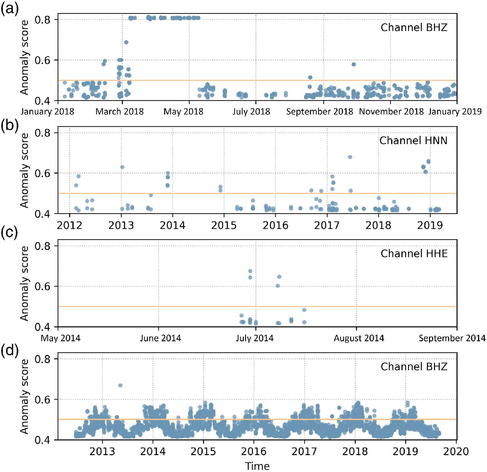Anomaly scores for four different channels (a) to (d). Each dot represents a recorded waveform segment of variable length

Notes:

This program uses a machine learning algorithm specifically designed for outlier detection (Isolation forest) where

• scores <= 0.5 can be safely interpreted in all applications as "no significant anomaly" (see Isolation Forest original paper - Liu et al. 2008 - for theoretical details)

• extreme score values are virtually impossible by design. This has to be considered when setting a user defined threshold T to discard malformed waveforms. In many application, setting T between 0.7 and 0.75 has proven to be a good compromise between precision and recall (F1 score)

• (Disclaimer) "False positives", i.e. relatively high anomaly scores even for well formed recordings have been sometimes observed in two specific cases:

  • recordings from stations with extremely and abnormaly low noise level (e.g. borhole installations)
  • recordings containing strong and close earthquakes. This is not a problem to check metadata errors, as the scores trend of several recordings from a given sensor / station will not be affected (except maybe for few sparse slightly higer scores), but has to be considered when filtering out segments in specific studies (e.g. with strong motion data): in this cases, setting a higher threshold is advisable. A model trained for accelerometers only (usually employed with these kind of recordings) is under study

Installation

Always work within a virtual environment. From a terminal, in the directory where you cloned this repository (last argument of git clone),

1. create a virtual environment (once). Be sure you use Python>=3.7 (Type python3 --version to check):

   python3 -m venv .env
   

2. activate it (to be done also every time you use this program):

   source .env/bin/activate
   

   (then to deactivate, simply type ... deactivate on the terminal).

   Update pip and setuptools (not mandatory, but in rare cases it could prevent errors during the installation):

   pip install --upgrade pip setuptools
   

3. Install the program (one line command):

   with requirements file:

   pip install -r ./requirements.txt && pip install -e .
   

   or standard (use this mainly if you install sdaas on an already existing virtualenv and you are concerned about breaking existing code):

   pip install "numpy>=1.15.4" && pip install -e .
   

   Notes:

   • The "standard" install actually checks the setup.py file and avoids overwriting libraries already matching the required version. The downside is that you might use library version that were not tested

   • -e is optional. With -e, you can update the installed program to the latest release by simply issuing a git pull

   • although used to train, test and generate the underlying model, scikit learn is not required for Security & maintainability limitations. If you want to install it, type pip install scikit-learn>=0.21.3 or, in the standard installation you can include scikit learn with pip install .[dev] instead of pip install .

     Due to the specific version to be installed, scikit might have problems installing.

     Few hints here:

     • you might need to preinstall cython (pip install cython)
     • you might need to brew install libomp, set the follwing env variables:

       export CC=/usr/bin/clang;export CXX=/usr/bin/clang++;export CPPFLAGS="$CPPFLAGS -Xpreprocessor -fopenmp";export CFLAGS="$CFLAGS -I/usr/local/opt/libomp/include";export CXXFLAGS="$CXXFLAGS -I/usr/local/opt/libomp/include";export LDFLAGS="$LDFLAGS -Wl,-rpath,/usr/local/opt/libomp/lib -L/usr/local/opt/libomp/lib -lomp"
       

     • and then install with the following flags:

       pip install --verbose --no-build-isolation "scikit-learn==0.21.3"
       

     (For any further detail, see scikit-learn installation page)

Run tests (optional)

python -m unittest -fv

(-f is optional and means: stop at first failure, -v: verbose)

Usage

sdaas can be used as command line application or as library in your Python code

As command line application

After activating your virtual environment (see above) you can access the program as command line application in your terminal by typing sdaas. The application can compute the score(s) of a single miniSEED file, a directory of miniSEED files, or a FDSN url (dataselect or station url).

Please type sdaas --help for details and usages not covered in the examples below, such as computing scores from locally stored files

Examples

Compute scores of waveforms fetched from a FDSN URL:

>>> sdaas "http://geofon.gfz-potsdam.de/fdsnws/dataselect/1/query?net=GE&sta=EIL&cha=BH?&start=2019-01-01T00:00:00&end=2019-01-01T00:02:00" -v
[████████████████████████████████████████████████████████████████████████████████████████████████████████]100%  0d 00:00:00
id start end anomaly_score
GE.EIL..BHN 2019-01-01T00:00:09.100 2019-01-01T00:02:12.050 0.45
GE.EIL..BHE 2019-01-01T00:00:22.350 2019-01-01T00:02:00.300 0.45
GE.EIL..BHZ 2019-01-01T00:00:02.250 2019-01-01T00:02:03.550 0.45

(note: The paremeter -v / verbose prints additional info before the scores table)

Compute scores from randomly selected segments of a given station and channel, and provide also a user-defined threshold (parameter -th) which will also append a column "class_label" (1 = outlier - assigned to the scores greater than the threshold and 0 = inlier)

>>> sdaas "http://geofon.gfz-potsdam.de/fdsnws/station/1/query?net=GE&sta=EIL&cha=BH?&start=2019-01-01" -v -th 0.7
[██████████████████████████████████████████████████████████]100%  0d 00:00:00
id start end anomaly_score class_label
GE.EIL..BHN 2019-01-01T00:00:09.100 2019-01-01T00:02:12.050 0.45 0
GE.EIL..BHN 2019-10-16T18:48:11.700 2019-10-16T18:51:02.300 0.83 1
GE.EIL..BHN 2020-07-31T13:37:19.299 2020-07-31T13:39:41.299 0.45 0
GE.EIL..BHN 2021-05-16T08:25:38.100 2021-05-16T08:28:03.150 0.53 0
GE.EIL..BHN 2022-03-01T03:14:23.300 2022-03-01T03:17:01.750 0.45 0
GE.EIL..BHE 2019-01-01T00:00:22.350 2019-01-01T00:02:00.300 0.45 0
GE.EIL..BHE 2019-10-16T18:48:18.050 2019-10-16T18:51:09.650 0.83 1
GE.EIL..BHE 2020-07-31T13:37:08.599 2020-07-31T13:39:28.499 0.45 0
GE.EIL..BHE 2021-05-16T08:25:49.150 2021-05-16T08:28:14.800 0.49 0
GE.EIL..BHE 2022-03-01T03:14:26.050 2022-03-01T03:16:41.900 0.45 0
GE.EIL..BHZ 2019-01-01T00:00:02.250 2019-01-01T00:02:03.550 0.45 0
GE.EIL..BHZ 2019-10-16T18:48:24.800 2019-10-16T18:50:47.300 0.45 0
GE.EIL..BHZ 2020-07-31T13:37:08.249 2020-07-31T13:39:30.199 0.45 0
GE.EIL..BHZ 2021-05-16T08:25:47.250 2021-05-16T08:28:10.850 0.47 0
GE.EIL..BHZ 2022-03-01T03:14:40.800 2022-03-01T03:16:53.900 0.45 0

Compute scores from randomly selected segments of a given station and channel, but aggregating scores per channel and returning their median:

>>> sdaas "http://geofon.gfz-potsdam.de/fdsnws/station/1/query?net=GE&sta=EIL&cha=BH?&start=2019-01-01" -v -agg median
[██████████████████████████████████████████████████████████]100%  0d 00:00:00
id start end median_anomaly_score
GE.EIL..BHN 2019-01-01T00:00:09.100 2022-03-01T03:17:45.950 0.46
GE.EIL..BHE 2019-01-01T00:00:22.350 2022-03-01T03:17:48.700 0.45
GE.EIL..BHZ 2019-01-01T00:00:02.250 2022-03-01T03:17:39.300 0.45

Same as above, but save the scores table to CSV via the parameter -sep and > (normal redirection of the standard output stdout to file)

>>> sdaas "http://geofon.gfz-potsdam.de/fdsnws/station/1/query?net=GE&sta=EIL&cha=BH?&start=2019-01-01" -v -sep "," > /path/to/myfile.csv
[████████████████████████████████████████████████████████████]100%  0d 00:00:00

in this case, providing -v / verbose will also redirect the header row to CSV. Note that only the scores table is output to stdout, everything else is printed to stderr and thus should still be visible on the terminal, as in the example above

As library in your Python code

This software can also be used as library in Python code (e.g. Jupyter Notebook) to work with ObsPy objects (ObsPy is already included in the installation): assuming you have one or more Stream or Trace, with relative Inventory, then

Compute the scores in a stream or iterable of traces (e.g. list. tuple, generator), returning the score of each Trace:

from obspy.core.inventory.inventory import read_inventory
from obspy.core.stream import read

from sdaas.core import traces_scores

# Load a Stream object and its inventory
# (use as example the test directory of the package):
stream = read('./tests/data/GE.FLT1..HH?.mseed')
inventory = read_inventory('./tests/data/GE.FLT1.xml')

# Compute the Stream anomaly score (3 scores, one for each Trace):
output = traces_scores(stream, inventory)

Then output is:

[0.45729656,  0.45199387,  0.45113142]

Compute the scores in a stream or iterable of traces, getting also the traces id (by default the tuple (seed_id, start, end), where seed_id is the Trace SEED identifier):

from obspy.core.inventory.inventory import read_inventory
from obspy.core.stream import read

from sdaas.core import traces_idscores

# Load a Stream object and its inventory
# (use as example the test directory of the package):
stream = read('./tests/data/GE.FLT1..HH?.mseed')
inventory = read_inventory('./tests/data/GE.FLT1.xml')

# Compute the Stream anomaly score:
output = traces_idscores(stream, inventory)

Then output is:

([('GE.FLT1..HHE', datetime.datetime(2011, 9, 3, 16, 38, 5, 550001), datetime.datetime(2011, 9, 3, 16, 42, 12, 50001)), ('GE.FLT1..HHN', datetime.datetime(2011, 9, 3, 16, 38, 5, 760000), datetime.datetime(2011, 9, 3, 16, 42, 9, 670000)), ('GE.FLT1..HHZ', datetime.datetime(2011, 9, 3, 16, 38, 8, 40000), datetime.datetime(2011, 9, 3, 16, 42, 9, 670000))], array([ 0.45729656,  0.45199387,  0.45113142]))

Same as above, with custom traces id (their SEED identifier only):

from obspy.core.inventory.inventory import read_inventory
from obspy.core.stream import read

from sdaas.core import traces_idscores

# Load a Stream object and its inventory
# (use as example the test directory of the package):
stream = read('./tests/data/GE.FLT1..HH?.mseed')
inventory = read_inventory('./tests/data/GE.FLT1.xml')

# Compute the Stream anomaly score:
output = traces_idscores(stream, inventory, idfunc=lambda t: t.get_id())

Then output is:

(['GE.FLT1..HHE', 'GE.FLT1..HHN', 'GE.FLT1..HHZ'], array([ 0.45729656,  0.45199387,  0.45113142]))

You can also compute scores and ids from iterables of streams (e.g., when reading from files)...

from sdaas.core import streams_scores
from sdaas.core import streams_idscores

... or from a single trace:

from sdaas.core import trace_score

For instance, to compute the anomaly score of several streams (for each stream and for each trace therein, return the trace anomaly score):

from obspy.core.inventory.inventory import read_inventory
from obspy.core.stream import read

from sdaas.core import streams_scores

# Load a Stream objects and its inventory
# (use as example the test directory of the package
# and mock a list of streams by loading twice the same Stream):
streams = [read('./tests/data/GE.FLT1..HH?.mseed'),
           read('./tests/data/GE.FLT1..HH?.mseed')]
inventory = read_inventory('./tests/data/GE.FLT1.xml')

# Compute Streams scores:
output = streams_scores(streams, inventory)

Then output is:

[ 0.45729656  0.45199387  0.45113142  0.45729656  0.45199387  0.45113142]

Same as above, computing the features and the scores separately for more control:

from obspy.core.inventory.inventory import read_inventory
from obspy.core.stream import read

from sdaas.core import trace_features, aa_scores

# Load a Stream object and its inventory
# (use as example the test directory of the package
# and mock a list of streams by loading twice the same Stream):
streams = [read('./tests/data/GE.FLT1..HH?.mseed'),
           read('./tests/data/GE.FLT1..HH?.mseed')]
inventory = read_inventory('./tests/data/GE.FLT1.xml')

# Compute Streams scores:
feats = []
for stream in streams:
    for trace in stream:
        feats.append(trace_features(trace, inventory))
output = aa_scores(feats)

Then output is:

[0.45729656, 0.45199387, 0.45113142, 0.45729656, 0.45199387, 0.45113142]

Maintenance

Although scikit learn is not used anymore for maintainability limitations, you can always consult the README explaining how to manage create new scikit-learn models.

Citation

Software:

Zaccarelli, Riccardo (2022). sdas - a Python tool computing an amplitude anomaly score of seismic data and metadata using simple machine‐Learning models. GFZ Data Services. https://doi.org/10.5880/GFZ.2.6.2023.009

Research article:

Riccardo Zaccarelli, Dino Bindi, Angelo Strollo; Anomaly Detection in Seismic Data–Metadata Using Simple Machine‐Learning Models. Seismological Research Letters 2021; 92 (4): 2627–2639. doi: https://doi.org/10.1785/0220200339